Assessing convergence

For a result to be valid, we need to ensure that longer simulation time would not result in different results, i.e., that our results are converged. The alchemlyb.convergence module provides functions to assess the convergence of free energy estimates or other quantities.

Time Convergence

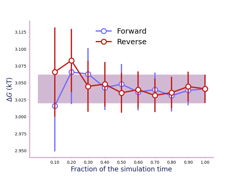
One way of determining the simulation end point is to compute and plot the forward and backward convergence of the estimate using forward_backward_convergence() and plot_convergence() [Klimovich2015].

>>> from alchemtest.gmx import load_benzene
>>> from alchemlyb.parsing.gmx import extract_u_nk
>>> from alchemlyb.visualisation import plot_convergence
>>> from alchemlyb.convergence import forward_backward_convergence

>>> bz = load_benzene().data
>>> data_list = [extract_u_nk(xvg, T=300) for xvg in bz['Coulomb']]
>>> df = forward_backward_convergence(data_list, 'mbar')
>>> ax = plot_convergence(df)
>>> ax.figure.savefig('dF_t.pdf')

Will give a plot looks like this

A convergence plot of showing that the forward and backward has converged fully.

Fractional equilibration time

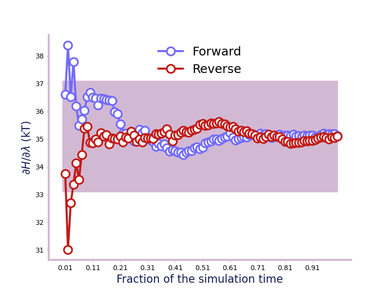
Another way of assessing whether the simulation has converged is to check the energy files. In [Fan2021] (and [Fan2020]), \(R_c\) and \(A_c\) are two criteria of checking the convergence. fwdrev_cumavg_Rc() takes a decorrelated pandas.Series as input and gives the metric \(R_c\), which is 0 for fully-equilibrated simulation and 1 for fully-unequilibrated simulation.

>>> from alchemtest.gmx import load_ABFE
>>> from alchemlyb.parsing.gmx import extract_dHdl
>>> from alchemlyb.preprocessing import decorrelate_dhdl, dhdl2series
>>> from alchemlyb.convergence import fwdrev_cumavg_Rc
>>> from alchemlyb.visualisation import plot_convergence

>>> file = load_ABFE().data['ligand'][0]
>>> dhdl = extract_dHdl(file, T=300)
>>> decorrelated = decorrelate_dhdl(dhdl, remove_burnin=True)
>>> R_c, running_average = fwdrev_cumavg_Rc(dhdl2series(decorrelated), tol=2)
>>> print(R_c)
0.04
>>> ax = plot_convergence(running_average, final_error=2)
>>> ax.set_ylabel("$\partial H/\partial\lambda$ (in kT)")

Will give a plot like this.

The A_c() on the other hand, takes in a list of decorrelated pandas.Series and gives a metric of how converged the set is, where 0 fully-unequilibrated and 1.0 is fully-equilibrated.

>>> from alchemlyb.convergence import A_c
>>> dhdl_list = []
>>> for file in load_ABFE().data['ligand']:
>>>     dhdl = extract_dHdl(file, T=300)
>>>     decorrelated = decorrelate_dhdl(dhdl, remove_burnin=True)
>>>     decorrelated = dhdl2series(decorrelated)
>>>     dhdl_list.append(decorrelated)
>>> value = A_c(dhdl_list, tol=2)
0.7085

Block Average

If one obtains suspicious results from the forward / backward convergence plot, it may be useful to view the block averages of the change in free energy using block_average() and plot_block_average() over the course of each step in lambda individually, the following example is for \(\lambda\) = 0

>>> from alchemtest.gmx import load_benzene
>>> from alchemlyb.parsing.gmx import extract_u_nk
>>> from alchemlyb.visualisation import plot_block_average
>>> from alchemlyb.convergence import block_average

>>> bz = load_benzene().data
>>> data_list = [extract_u_nk(xvg, T=300) for xvg in bz['Coulomb']]
>>> df = block_average(data_list, 'mbar')
>>> ax = plot_block_average(df)
>>> ax.figure.savefig('dF_t_block_average.png')

Will give a plot looks like this

A plot of the free energy divided into block averages showing consistency/inconsistency across the trajectory.

Convergence functions

Convergence functions are available from alchemlyb.convergence. Internally, they are imported from submodules, as documented below.

convergence

Functions for assessing convergence of free energy estimates and raw data.